The Challenge

I wanted to write a program to identify a map of a US state.

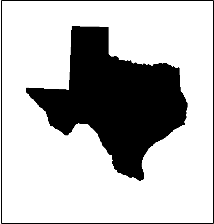
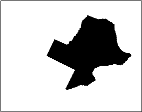
To make life a little more challenging, this program had to work even if the maps are rotated and are no longer in the standard “North is up” orientation¹. Further the map images may be off-center and rescaled:

Data Set

The first challenge was getting a set of 50 solid-filled maps, one for each of the states. Some Google searching around led to this page which has outlined images for each state map. Those images have not just the outline of the state, but also text with the name of the state, the website’s URL, a star showing the state capital and dots indicating what I assume are major cities. In order to standardize the images, I removed the text and filled in the outlines. The fill took care of the star and the dots.

First some Python to get the list of all state names:

1
2
3
4
5
6
7
8
9
10
11

text = requests.get("http://www.50states.com/us.htm").text
doc = lxml.html.document_fromstring(text)

states = []
for a in doc.findall(".//ul[@class='bulletedList']/li/a"):
    url = a.get("href")
    state_name = posixpath.splitext(posixpath.split(urlparse.urlsplit(url).path)[-1])[0]
    states.append(state_name)

def make_url(state):
    "return http://www.50states.com/maps/%s.gif" % state

Next I tried to open one of these images using OpenCV’s imread only to discover that OpenCV does not handle gifs so I built this utility method to convert the GIF to PNG and then to read them with imread:

With the images loaded, I believed the following operations should suffice to get my final, filled-in image:

1. Remove the text heading (strip off some number of rows from the top of each image).
2. Convert “color” image to binary image (1=black, 0=white) (this will be required by findContours)
3. Find the “contours” that bound areas we will fill in (i.e. identify the state outlines).
4. Convert contours to polygons.
5. Fill in area bounded by “significant” polygons.

Here when I say significant polygons, I want to make sure the polygon bounds a non-trivial area and is not a stray mark.

I use the following methods to convert image and to display the image using matplotlib:

This is my first attempt at the algorithm:

Which seems to work for most states, but fails for Massachusetts:

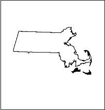
This seems to be due to a break somewhere in the outline. A simple dilate with a 3x3 kernel solved the problem.

The final algorithm is here:

which works for all states:

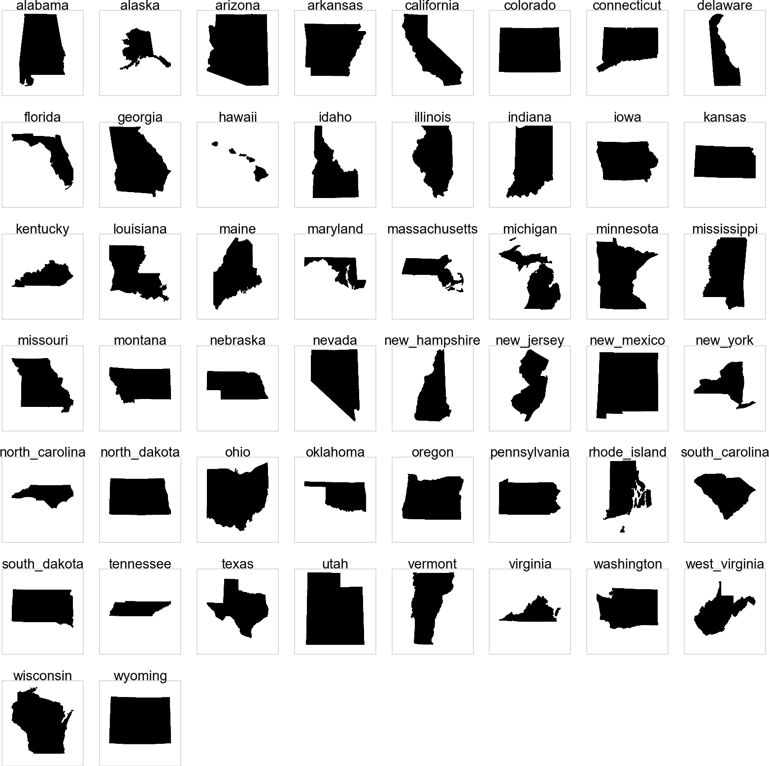
Image Recognition

I needed some way of comparing two images which may have different rotations, scalings and/or translations. My first thought was to develop a process that normalizes an image to a canonical orientation, scaling and position. I could then take an unlabeled image, and compare its standardized form to my set of canonicalized maps pixel-by-pixel with some distance metric such as MAE or MSE.

How to normalize the image? Image moments immediately came to mind. The zeroth moment is the “mass” of the image (actually the area of the image since I am working with black and white images, where the black pixels have unit mass and the white pixels to have no mass). The area can be used to normalize for image scaling.

The first moment is the center of mass or the centroid of the image. Calculating the centroid is then an arithmetic average of black pixel coordinates. The center of mass is a reference point and that allows me to normalize for translation of the image. Finally, I would like an “axis of orientation” which I can used to normalize rotation. Wikipedia provides the answer but a more complete explanation can be found here.

At this point I realized that rather than going through the trouble of standardizing the image and then comparing pixel-by-pixel, I could just compare a set of so-called “rotation invariant moments”. These values are invariant for a given image under translation, scale and rotation. OpenCV provides a function to calculate the Hu moments. The Hu moments are the most frequently used, but Flusser shows there are superior choices. For convenience I will use the seven Hu moments as feature values in a machine learning classifier.

In order to classify the images using the seven feature values, I decided to use scikit-learn’s SVM Classifier. I generated training data by taking each of the 50 state images, and then rotating, shifting and scaling them and then getting the Hu moments for the resulting image. I took this set of examples, split 20% out as test data and 80% for training. After observing that each of the seven features takes on very different ranges of values, I made sure to scale my features.

An SVM with a linear kernel resulted in 31% classification accuracy. This is certainly better than the 2% I would get from blind guessing but a long way from what a gifted elementary school student would get after studying US geography. Using an “rbf” kernel and a default setting for gamma gives an accuracy of 20%. With some tweaking to gamma, I was able to get this up to 99%, but this required a gamma=10000. Having this large a gamma made me question my approach. I reviewed the OpenCV method matchShapes which also uses the Hu Moments. I noticed that rather than just comparing the Hu Moments, the OpenCV method instead compared the log of the moments.

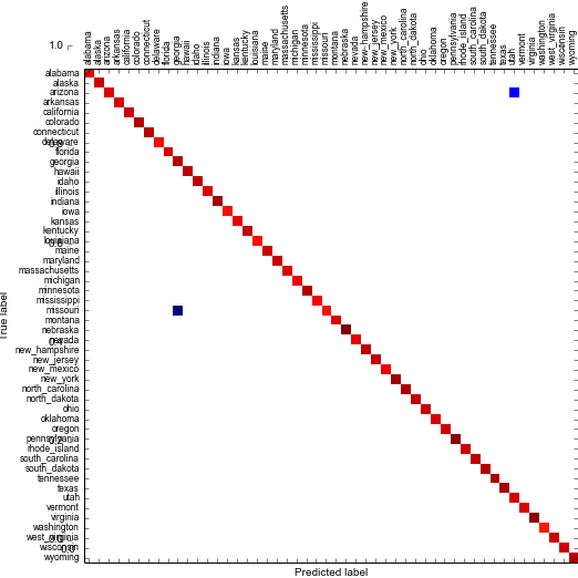
I changed my features to be the signum’ed log of the absolute values of the Hu Moments, and then applied standard scaling. This log transform of the Hu moments is pretty common in the literature, see: Conley². After doing that my linear kernel SVM was able to achieve a score of 100%. An rbf kernel with default gamma got a score of 99% (looking at the confusion matrix shows some confusion between Utah vs. Arizona and Georgia vs. Missouri, which do look similar):

Blurring

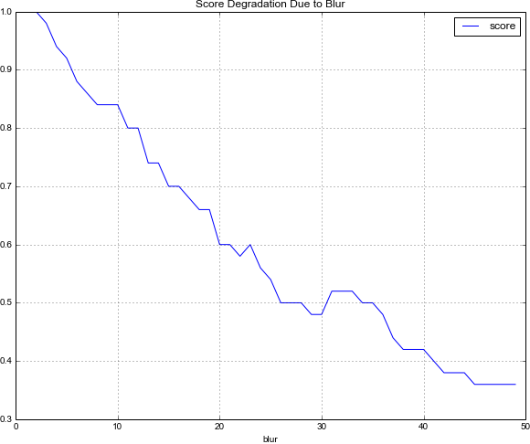
While not part of the original problem specification, I wanted to see how this classification technique would fare under image blurring. I show below classification scores as a function of increasing amounts of blur. Using a normalized box filter:

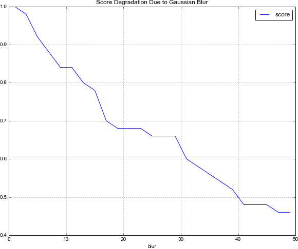
and a Gaussian Blur:

My IPython Notebook is available here.

Extensions

It would be cool to evaluate this same technique on maps of countries. I have found two source of country maps: this and this. Using the second link, the URLs for the country pages can be extracted using:

1
2
3
4
5
6
7
8
9
10

text = requests.get("http://www.worldatlas.com/sitemap.xml").text
el = lxml.etree.fromstring(str(text))

urls = []
for url in el:
    urls.append(url[0].text)

series = pd.Series(urls)
series = series[series.str.contains("outline") & series.str.contains("countrys")]
series = series[~series.str.contains("states") & ~series.str.contains("province")]